Code: https://github.com/LEGO999/A-tutorial-for-few-shot-learning
Prof. Shusen Wang at the Stevens Institute of Technology provided an informative tutorial for few-shot learning and metric learning. I took lecture notes and complemented this tutorial with additional materials and code built on PyTorch.
Definition of few-shot learning
Few-shot learning aims to empower machine learning methods to generalize via providing a few samples.
N-way K-shot learning
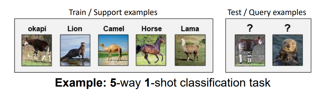
Fig.1 An example (source: CVPR 2020 Tutorial: Towards Annotation-Efficient Learning )
- N = number of classes in the support set
- K = training examples per class, as small as 1 or 5
Training
Dataset
| Meta-training | Meta-test | |||
|---|---|---|---|---|
| Training | Support | Query | Support | Query |
- Training set, support set, and query set do not have any intersection of classes.
- The goal of the few-shot learning: learn a similarity function on base classes in the training set to find the sample(s) in the query set, which is (are) similar to those in the support set.
- Common datasets: Omniglot, MiniImageNet, CUB, ImageNet-FS, CIFAR-FS
How do they work
- Metric learning: Siamese Network, Triplet loss, Match Network, cosine distance based classifier.
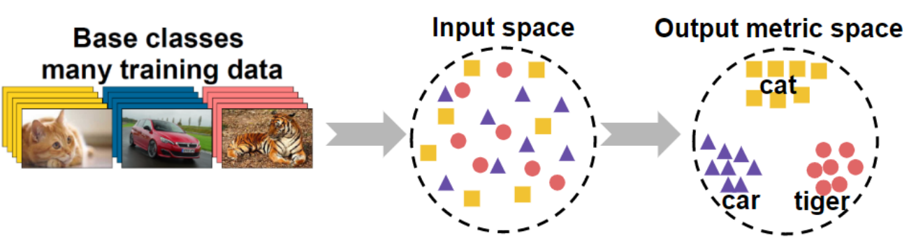
Fig.2 An illustration of metric learning (source: CVPR 2020 Tutorial: Towards Annotation-Efficient Learning )
- Meta-learning:
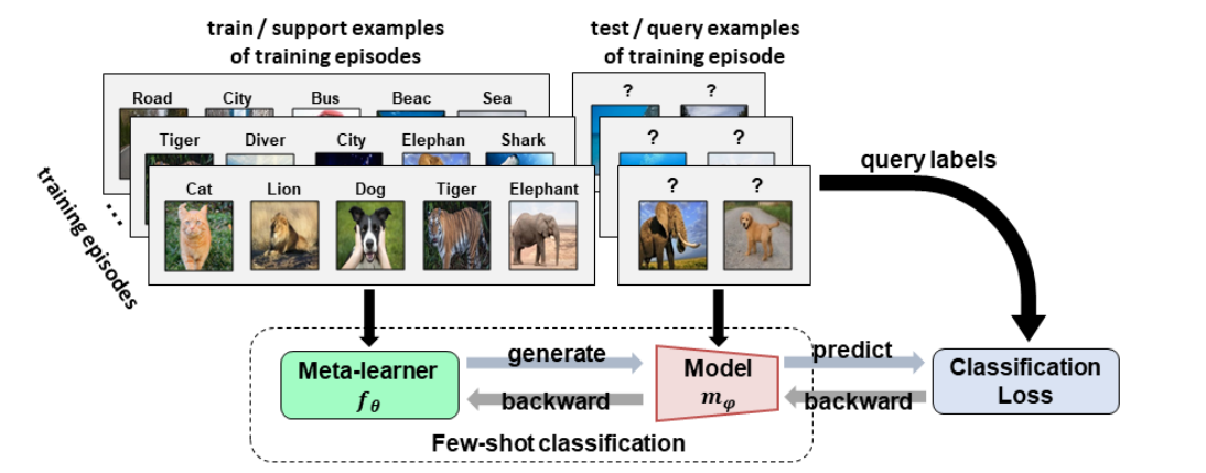
Fig.3 Training stage of meta-learning (source: CVPR 2020 Tutorial: Towards Annotation-Efficient Learning )
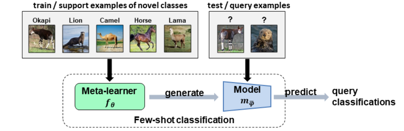
Fig.4 Testing stage of meta-learning (source: CVPR 2020 Tutorial: Towards Annotation-Efficient Learning )
Test
- Get embeddings from backbone for support samples and query samples
- Calculate the cosine similarity between two kinds of embeddings.
- $\text{cos}\ {\theta} = \frac{X^{T}W}{\lVert X \rVert_{2} \lVert W \rVert_{2}}$, where $X$ and $W$ are embeddings.
- By using cosine similarity, we focus on angular difference rather than amplitudes of $X$ and $W$.
- Get probability via
softmax()the similarity.
Translate these steps to PyTorch code, and they look like:
def embedding2prob(query_out, support_out):
    query_batch_size = query_out.shape[0]
    # repeat embedding according to the number of ways
    query_out = query_out.repeat_interleave(support_out.shape[0] // query_batch_size,0)
    sim = F.cosine_similarity(query_out, support_out).view(query_batch_size, -1)
    prob = F.softmax(sim, dim=-1)
    return prob
Examples of metric learning methods
Siamese network
Siamese network learns a pairwise similarity function as depicted in Fig.5. If two samples come from the same class, they will marked as a positive training pair. If two samples come from two different classes, they will be marked as a negative training pair.
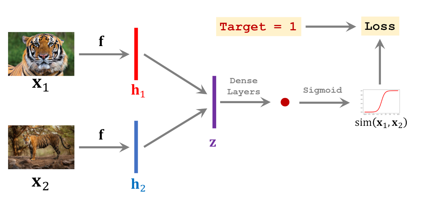
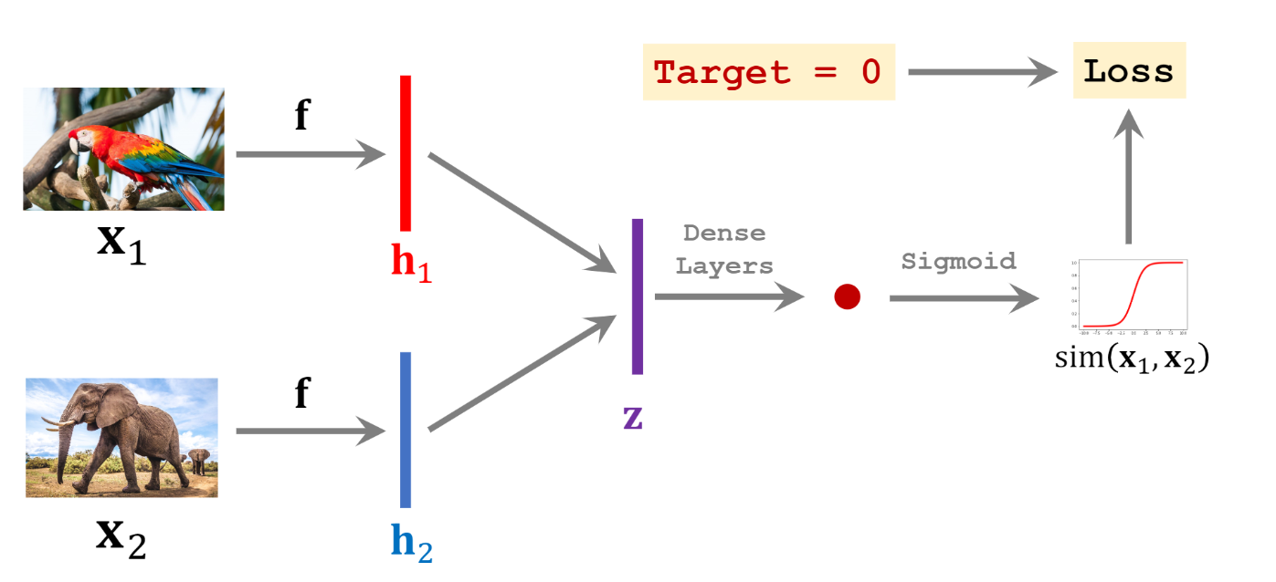
Fig.5 Positive and negative training samples of a Siamese network (source: Shusen Wang: Deep Learning )
Triplet network
Triplet network extends the idea of the Siamese network into a three-sample combination. As described in Fig.6, a triplet network tries to decrease the $l_{2}$-distance $d^{+}$ between embeddings of the positive sample and the anchor sample, as well as increase the $l_{2}$-distance $d^{-}$ between embeddings of the negative sample and the anchor sample. To be specific, a triplet network makes $d^{+} - d^{+} >= a$, where $a$ is a user-defined margin.
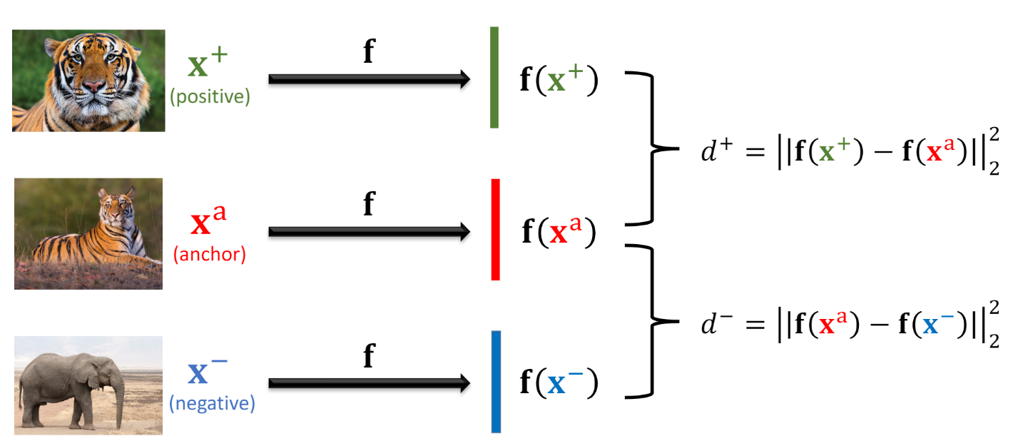
Fig.6 Triplet loss (source: Shusen Wang: Deep Learning )
The loss itself is relatively easy to implement. For numerical stability, I suggest to use PyTorch’s built-in loss function torch.nn.TripletMarginLoss().
The point of implementation is to let our data loader sample anchor positive and negative samples simultaneously. I implement this feature via torch.utils.data.Sampler as follows.
# sample anchors, positive and negative samples for triplet loss
class TripletBatchSampler(torch.utils.data.Sampler):
    def __init__(self, dataset, batch_size):
        self.dataset = dataset
        self.batch_size = batch_size
        # obtain labels for all samples sequentially
        self.label = [label for _, label in self.dataset._flat_character_images]

    def __iter__(self):
        indices = list(range(len(self.dataset)))
        # obtain indices of samples and their corresponding labels
        target_with_indices = list(zip(indices, self.label))
        # shuffle data
        random.shuffle(target_with_indices)
        num_class = max(self.label)+1
        # obtain indices of samples from each class and save into the dictionary
        class_dict = {k: [] for k in range(num_class)}
        for (sample_idx, class_idx) in target_with_indices:
            class_dict[class_idx].append(sample_idx)

        for k in range(len(self)):
            offset = k * self.batch_size
            # sample anchors and get their labels
            anchor_indices, class_indices = zip(*target_with_indices[offset:offset+self.batch_size])
            anchor_indices = list(anchor_indices)
            positive_indices = []
            negative_indices = []
            for class_idx in class_indices:
                # sample a postive sample which have the same classes as the anchor
                positive_indices.append(random.choice(class_dict[class_idx]))
                # create a list which excludes the anchor class
                absent_list = list(range(num_class))
                absent_list.remove(class_idx)
                # choose a negative class randomly
                negative_class = random.choice(absent_list)
                # sample a negative samples from the chosen negative class
                negative_indices.append(random.choice(class_dict[negative_class]))
            yield anchor_indices + positive_indices + negative_indices

    def __len__(self):
        return len(self.dataset) // self.batch_size + 1
Additional experiments
I use a ResNet-18 and the Omniglot dataset to validate my implementation. Data of Omniglot are normalized to mean of zero and standard derivation of one. Here, I use SGD optimizer with an initial learning rate of 0.1. All networks are trained for 30 epochs,and the learning rate drops by $10\times$ at epoch 24 and 27. The DNN in experiment 0 is trained from scratch using Triplet Loss. In experiments 1, 2, and 3, DNNs are pre-trained on CIFAR-10. In experiment 1, no additional training is adopted. In experiment 2, the DNNs are frozen by the 13th Conv layer; other layers are fine-tuned by Triplet Loss. In experiment 3, a normal supervised classification head (an FC layer + softmax) is attached. The DNN is trained by the cross-entropy loss. Similar to the previous experiments, only the embeddings of the Conv net will be utilized for the few-shot evaluation. All DNNs are evaluated on the test set of Omniglot at the beginning of the epoch.
| Experiment | Training methods | Loss | Few shot accuracy (%) | |||
|---|---|---|---|---|---|---|
| Pre-trained | Frozen by conv13 | Unfrozen | Triplet | Supervised | ||
| 0 | $\textbf{X}$ | $\textbf{X}$ | 94.83 | |||
| 1 | $\textbf{X}$ | 47.95 | ||||
| 2 | $\textbf{X}$ | $\textbf{X}$ | $\textbf{X}$ | 82.68 | ||
| 3 | $\textbf{X}$ | $\textbf{X}$ | $\textbf{X}$ | 91.66 | ||